
How to Calculate Percentage Change Between Two numbers in Excel.
If you work with numbers in Microsoft Excel, it is very likely that you need to calculate percentage changes regularly. Fortunately, Excel provides several formulas and techniques to help you easily calculate the percentage change or the difference between two numbers or cells and we will present them in this tutorial.
Percentage change, also known as percentage variation or difference, is used to show the difference between two values. In other words, the percentage change is a way of telling how much something has increased or decreased in percentage terms, compared to its previous value.
For example, you can use it to determine the percentage increase or decrease in the number of students in a school between last year and this year, or the price difference in a product compared to last month, or the number of website visitors before and after the implementation of a marketing campaign, etc.
In this article, I will show you how to calculate the percentage change between two numbers in Excel, and how to count the percentage change when you have negative or zero values.
- Find Percentage Change in Excel.
- Formatting the Percentage Result (Decimal places, Color).
- Find Percentage Change when having Negative Values.
- Working with Percentage Change and Zero values.
- Count Percentage Change between Cells in the Same Column.
- Find Percentage Change to a Reference number/value.
How to Count Percentage Increase or Decrease in Microsoft Excel.
Finding the percentage change between two numbers in Excel is not difficult and can be done by using one of the following two (2) formulas:
- =(new_value–old_value)/old_value
- =(new_value/old_value)–1
Where:
● new_value: refers to the most recent or final value of the two numbers being compared.
● old_value: is the initial value between the two numbers compared to calculate the percentage change.
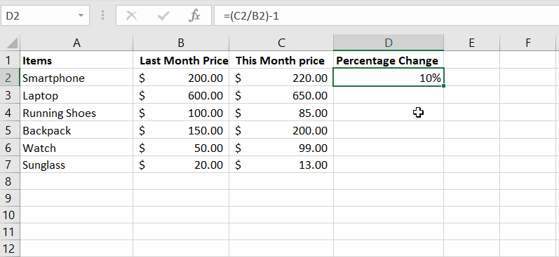
Example: Suppose you want to know what percentage (in percent) the price of a list of products has increased or decreased since the previous month. To complete this task, you need to calculate the percentage change of each product between its current price (new_value) and its previous price (old_value).
1. Open a new spreadsheet in Excel.
2. Type your column headings in cells in first row as follows:*
- In the first column in cell A1 type "Items" for the product description.
- In the second column in cell B1 type "Last Month Price" ("old_value").
- In the third column in cell C1 type "This month price" (new_value")

3. Now, under each heading, enter the relevant information, (i.e. the description of the product, the price of the previous month and the price of the current month).

4. Optionally: After filling in the prices of the products, you can, if you wish, specify the type of currency (e.g. dollars ($), euros (€), etc.), as follows:
Click on one of the letters of the columns with the prices (e.g. "B"), and then in the Home tab click the arrow next to the dollar $ and choose the currency format [e.g. "$ English (United States)].

5. Then, at the first cell of the first empty column (e.g. the "D1" in this example), type "Percentage Change".
6. Now use one of the two (2) methods/formulas below to find the percentage change.
Method A. Calculate Percentage Change with: =(new_value–old_value)/old_value"
To count the percentage in our example using the formula:
=(new_value–old_value)/old_value
a. Select the first empty cell under the "Percentage Change" (e.g. the cell "D2), type the below formula and press Enter (or click in one empty cell). *
=(C2-B2)/B2
* Note: Here, the old value (B2) is subtracted from the new value (C2) and the result is divided by the old value (B2).

b. After pressing Enter, the percentage change will be in decimal values as shown below. To change the result to percentage format, select the cell D2 and click the Percentage style button (%) in the Number group.
* Note: You can also apply Percentage formatting to the result cell before entering the formula.

c. Now, you have the percentage change between the two values in cells B2 & C2, in cell D2 which is 10%.

6. After calculating the percentage change for the first product (e.g. "the "Smartphone" in this example), we can apply the same formula to view the percentage change for all the other items. To do that:
Click and drag the Fill handle (the small green square located at the lower right corner of the formula cell) downwards to copy the formula across the cells you wish to fill.


Method B. Calculating the Percentage Change with: =(new_value/old_value)–1"
The second method to find out the percentage change in Excel is by using the formula:
=(new_value/old_value)–1
e.g. To find the percentage change between the two values in cells B2 and C2, type the following following formula:
=(C2/B2)-1

As you can see, the second formula can give us the same result as the first formula. Copy the formula to the rest cells below for all the products and you're done!

How to Format Decimal Places and Color of the Result percentage.
As you will see in our example, the percentage result is displayed without decimal places and with a negative sign when there is a percentage decrease.

If you want to display the exact percentage increase or decrease (i.e. with decimal places) and format e.g. the negative percentages in a different color (eg red), so that you can easily understand the difference, do the following:
1. Select all the cells with the percentage change, then right-click and select Format Cells from the context menu.

2. In the "Format Cells" window, click on the Custom option on the left menu, type the below code in the Type: text field and click OK. *
0.00%;[Red]-0.00%
* Notes:
1. If you using the Comma (,) as a decimal symbol, replace the dot (.) with the comma (,). e.g.: "0,00%;[Red]-0,00%"
2. To format the positive percentage change in e.g. "Green" color and the negative with "Red" type: "[Green]0.00%;[Red]-0.00%"

3. This will format all the decreasing percentage changes in red color and will also display two (2) decimal places for exact percentages.

How to Calculate the Percentage Change when having Negative Values.
If you have some negative numbers in your values, the regular percent difference formula may not give you the correct result. More specifically:
● If both the old and new values are negative or positive, you can use the percentage formulas without any issues.
● If the old value is positive and the new value is negative, you can also use the given percentage formulas to get the correct answer.
● But, if the old value is negative and the new value is positive, the percentage formula will give you wrong result, as you can see at cells "C4" & "C7" in the screenshot below.

To fix this issue, insert the "ABS" function to make the denominator a positive number, by using and applying this formula to all percentage cells:
=(new_value – old_value) / ABS(old_value)
* Note: This will ensure that the formula works correctly no matter which value is a negative number).
e.g. In our example, the formula will be: "=(B1-A1)/ABS(A1)"

How to Find the Percentage Change when having values with Zero(s)
If your cells contain zero values in either the old or new value, you may encounter an #DIV/0! error message. This happens because you cannot divide any number by zero in math.

To fix this issue, you can insert the "IFERROR" function in your Excel formula, so if the percent change formula encounters any error (e.g. the "#DIV/0!" error), will return "0%" as a result:*
=IFERROR((new_value – old_value) / ABS(old_value),0)
* Note: If you using the Comma (,) as a decimal symbol, replace the Comma ","in the formula with a Semicolon ";" and use the below formula:
=IFERROR((new_value – old_value) / ABS(old_value);0)
e.g. In our example (where we use the Comma (,) as a decimal symbol), the formula will be: "=IFERROR((B1-A1)/ABS(A1);0)"

How to calculate the percentage change between cells of the same column.
The way to measure the percentage change between cells in the same column is almost the same as described above for measuring the percentage change between cells in the same row.
Example: To calculate the percentage increase or decrease of your profits from month to month.
1. Open a blank Excel document and enter e.g. the months and their profit.

2. Then select an empty cell where you want to display the percentage change between the first two months (e.g. the "C3" in this example) and type this formula to count the percentage change between the first two months (January & February): *
=(B4-B3)/B3
* Where: B4 = the second month's earnings, and B3 = the first month's earnings.

3. Next, apply the formula to the rest columns (C3 to C14) and then, if you want, apply also the custom color formatting (as described above) for the negative percentages.

How to Find Percentage Change to a Reference value.
If you want to calculate the percentage change relative to a specific cell (reference value), add the "$" sign before both the column letter and row number of the reference cell.
Example: To calculate the percentage change in profit for February (B4) compared to January (B3) as the reference month, the formula is:
=(B4-$B$3)/$B$3

Then, apply the formula to the rest of the cells to get the percentage change for each other month compared to January.

That's it! Let me know if this guide has helped you by leaving your comment about your experience. Please like and share this guide to help others.

- How to Resolve Hyper Backup Error "Failed to Export System Configuration" on Synology NAS. - June 17, 2026
- How to Require MFA for All Users in Microsoft 365 with a Conditional Access Policy. - June 15, 2026
- How to Resolve Error "Something Went Wrong 657rx" in Outlook or Microsoft 365 Apps. - June 10, 2026


