How to Find and Remove Duplicates in Excel.
If you are looking for easy ways to find and remove duplicate entries in Excel, you are in the right place because, in this guide, we will walk you through easy methods of doing so in detail.
Microsoft Excel is widely used, but it can be confusing when data is repeated, as this reduces the practicality of spreadsheets. Incorrectly creating duplicate records in Excel can lead to inaccurate reports and skewed measurements, thus making the results unreliable.
Fortunately, finding and removing duplicates in Excel is quite simple. You will find several ways to accomplish this task below, so let's get started.
How to Find & Remove Duplicate Entries in Excel.
- Method 1. Highlight & Remove Duplicates in Excel.
- Method 2. Delete Duplicates in Excel using "Remove Duplicates" command.
- Method 3. Hide Duplicates entries in Excel.
- Method 4. Remove Duplicate Values with Power Query Tool.
- Method 5. Remove Duplicates in Excel with a Formula.
Method 1. How to Find and Highlight Excel Duplicate entries.
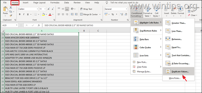
An easy way to find and delete the duplicate values in Excel is to highlight and remove them manually, by using the Conditional Formatting feature.
1. Select the cell(s), or column(s) from which you want to remove duplicates.
2. Now in the Home tab, click on Conditional Formatting and select Highlight Cells Rules –> Duplicate Values.
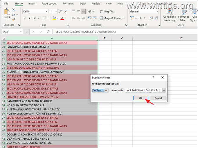
3. A dialogue box should pop up on your screen now. Pick if you want a different color for the duplicate values (in the box next to "values with"), and then click OK.
4. Once the duplicate entries are identified, you can manually remove them easily.
Method 2. How to Delete Excel Duplicate entries with "Remove Duplicates" command.
The easiest way to remove the duplicate values in a Excel file, is through the ‘Remove Duplicates’ command within the program.
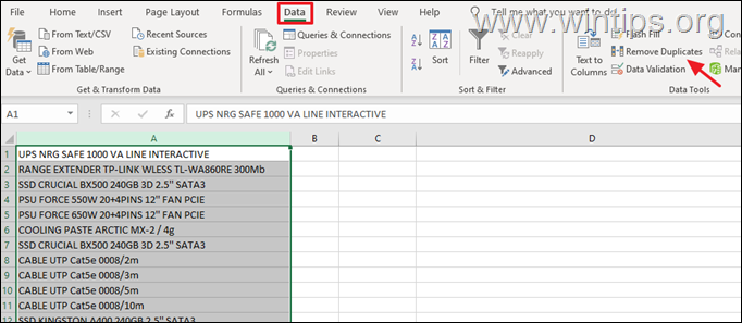
1. In Excel file, select the cell(s) or column(s) from which you want to remove duplicates.
2. Head over to the Data tab and then select Remove Duplicates.
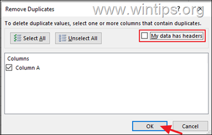
3a. This should open the Remove Duplicates window. Here, you can choose from which columns you want to remove duplicate values and if you data has headers or not.*
* Note: If your data has headers leave the corresponding checkbox checked.
3b. When done hit OK.
3c. After that you'll be informed how many duplicate entries found and removed and how many unique entries remain.
Method 3. How to Hide Excel Duplicate Values using Advanced Filters.
1. Select the cell(s), or column(s) from which you want to remove duplicates.
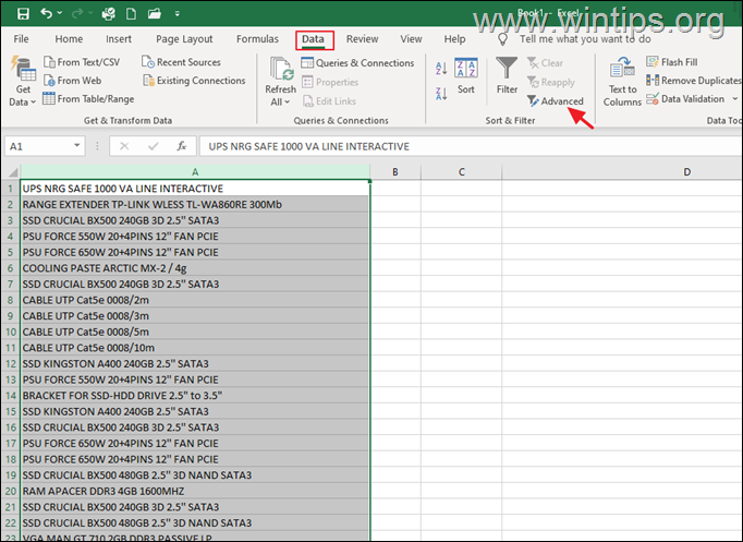
2. From the Data tab, click Advanced to open the filters window.
3. In Advanced Filter window, choose the following and click OK:
- Filter the list, in-place.
- Unique records only.
4. When the list is filtered in place, the duplicate rows will be hidden, but when the data is copied to another location, the duplicate rows will be removed.
Method 4. How to Remove Excel Duplicates using the Power Query Tool
1. Launch Excel and select the cells/range of cells that you want to check for duplicates.
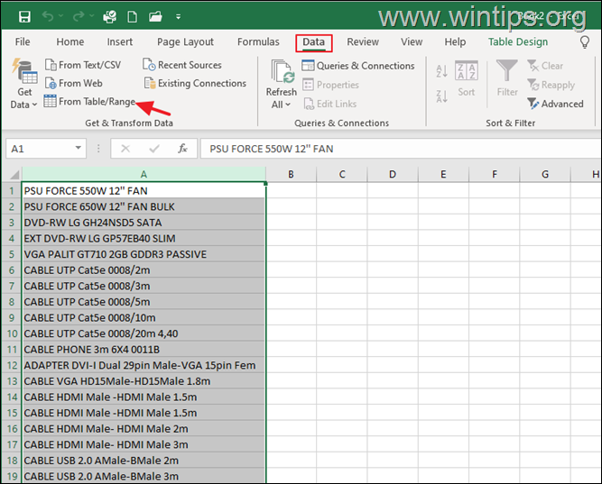
2. Now head over to the Data tab and click on From Table/Range. Hit OK in the Create Table dialogue box.
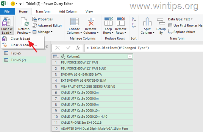
3. In Power Query Editor, right-click on the column that you want to remove the duplicates and select Remove Duplicates.
4. Click Close & Load from the menu to create a new sheet inside the current workbook with the unique entries.
Method 5. How to Remove Duplicate Entries in Excel using a Formula.
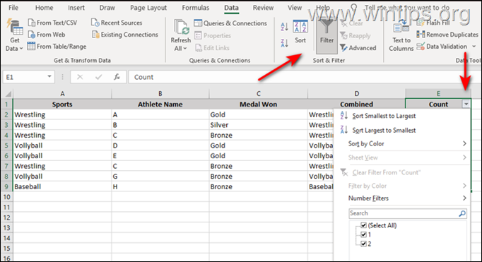
To illustrate this approach, we will use a simple example with columns called "Sports", "Athlete's name" and "Medal won" which we will combine into a new column called "Combined". So, lets start.
1. Select the first empty cell in "Combined" column (e.g. "D2" in this example) and type the formula for the combination of the 3 first columns in the formula bar. (e.g. "=A2&B2&C2" in this example). When done, press Enter.
2. Then copy the formula down to all the rows. It should automatically modify according to the number of rows.
3. Now create another column and name it ‘Count’. This column will help identify the duplicate values.
4. At the first empty cell of "Count" column (e.g. "E2") use the COUNTIF function and type this formula:
=COUNTIF($D$2:D2,D2)
5. Copy the above formula down to all the rows.
6. Now, if the value of Count is “1”, then it has only appeared once and is unique. If the value is “2” or more, then it is considered a duplicate value.
6. Now select the Count column and head over to the Data tab.
7. Select Filter and click on the arrow icon against your column.
8. Only keep the box against 1 check-marked. Uncheck the rest and hit OK. This should remove the duplicate values.
That's it! Which method worked for you?
Let me know if this guide has helped you by leaving your comment about your experience. Please like and share this guide to help others.
- FIX: Device encryption is temporarily suspended and does not resume after the computer restarts (Windows 11). - May 5, 2026
- How to Install Chrome or any 'Line of Business' app on Intune Enrolled Windows Devices. - April 29, 2026
- How to Create a DDM Update Policy for iOS Devices in Intune. - April 23, 2026









February 19, 2024 @ 11:20 am
Great job! This is written to be very amazing and filled with the necessary words.